A mysterious constant called pi, arising from the Gaussian integral (with a minor application to circles)

Hi, nerd blog! (This is a post that I wrote a long time ago and then never published. I figured it would be nice to publish it on March 14th.)

Today, we’re interested in the Gaussian integral

$f(C) := \int_{-\infty}^\infty e^{-Cx^2} {\rm d} x$

for $C > 0$ . This integral of course has lots of very serious practical applications, as it arises naturally in the study of the Gaussian/normal distribution. But, more importantly, it’s a lot of fun to play with and is simply beautiful. We’ll see a bit about what it makes it so pretty below. We start by simply trying to figure out the value of this thing, which isn’t super easy.

By a change of variables, we immediately see that $f(C)$ is proportional to $1/\sqrt{C}$ . But, what is the constant of proportionality? It’s actually nicer to ask a slightly different question: what is the unique value of $C$ such that $f(C) = 1$ . A quick numerical computation shows that $f(3.14159) \approx 1$ . E.g., here’s some Mathematica code to find this value:
.

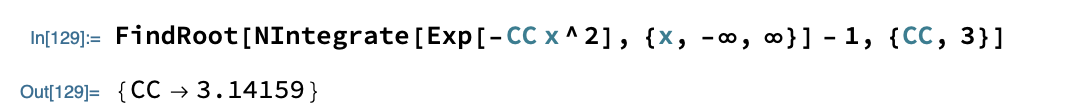This constant $C \approx 3.14159$ is so important for this blog post that it is worth giving it a name. So, I looked through the Greek alphabet for a nice letter that doesn’t get used much and chose the obscure lowercase letter $\pi$ —spelled pi in English, and pronounced like “pie”. In other words, by definition $f(\pi) = 1$ . (If this implicit definition bothers you, we can equivalently just define $\pi := f(1)^{2}$ . But, I find the implicit definition to be more elegant.)

So, we have this brand new mysterious constant $\pi$ . What should we do with it? It is of course natural to try to find different expressions for it (though our integral expression can already be used to compute it to quite high precision). A first idea is to apply the change of variables $u = \pi x^2$ to obtain

$1 = 2\int_{0}^{\infty} e^{-\pi x^2}{\rm d} x = \pi^{-1/2} \int_0^{\infty} e^{-u}/u^{1/2} {\rm d} u\; .$

So,

$\pi =\Big( \int_0^\infty e^{-u}/u^{1/2} {\rm d} u\Big)^2\; ,$

which you might recognize as the square of the Gamma function evaluated at $1/2$ , i.e., $\pi = \Gamma(1/2)^2$ . (Recalling that $\Gamma(n) = (n-1)!$ for integer $n$ , one might interpret this as saying that $\sqrt{\pi}$ is “the factorial of $-1/2$ .”)

This mysterious identity will play a key role later. We could, of course, find other identities involving this new constant $\pi$ . But, I thought instead I’d jump ahead to a rather obscure fact about the relationship between $\pi$ and a circle.

Our constant’s relationship with circles

In my opinion, the Gaussian distribution is far more interesting in dimensions larger than one. In particular, consider the distribution on $\mathbb{R}^n$ given by the probability density function

$\Pr[\mathbf{x}] = e^{-\pi \|\mathbf{x}\|^2}\; .$

Notice that

$\int_{\mathbb{R}^n}e^{-\pi \|\mathbf{x}\|^2} {\rm d} \mathbf{x} = \int_{-\infty}^{\infty} \cdots \int_{-\infty}^{\infty} e^{-\pi x_1^2 -\cdots - \pi x_n^2} {\rm d}x_1 \ldots {\rm d} x_n = 1\; ,$

so that this is in fact a distribution.

In fact, up to scaling, this distribution is the unique continuous radial product distribution—i.e., the unique distribution such that $\Pr[\mathbf{x}]$ can be written both as a function only of the norm of $\mathbf{x}$ , $\Pr[\mathbf{x}] = f^*(\|\mathbf{x}\|)$ for some continuous function $f^*$ , and as a product of functions of its coordinates, $\Pr[\mathbf{x}] = f_1(x_1)\cdots f_n(x_n)$ . This makes the Gaussian a uniquely powerful tool for reducing complicated multi-dimensional problems to one-dimensional problems.

For example, suppose that for some strange reason we wish to know the circumference of a circle with radius one. (If we were less civilized mathematicians, we might instead set the diameter to be equal to $1$ , so that the radius would be $1/2$ .) We can try to write this as some kind of path integral or something—and suffer quite a bit in the process—or we can use the following beautiful trick. We can write

$1 = \int_{\mathbb{R}^2} e^{-\pi \|x\|^2} {\rm d} x = \int_0^\infty e^{-\pi r^2} \sigma_r {\rm d} r= \sigma_1 \int_0^\infty e^{-\pi r^2} r {\rm d} r\;,$

where $\sigma_r$ is the circumference of a circle of with radius $r$ . (The only facts that we have used here are our definition of $\pi$ together with the fact that $\sigma_r = r \sigma_1$ .) Fortunately, the last integral is easy to compute as

$\int_0^\infty e^{-\pi r^2} r {\rm d} r = \frac{1}{2\pi} \cdot \int_0^\infty e^{-u} {\rm d} u = \frac{1}{2\pi} \;.$

Rearranging, we see that $\sigma_1 = 2\pi$ !

So, surprisingly, our mysterious constant $\pi$ is actually intimately related with the circumference of a circle. (If we were less civilized mathematicians, we might even have simply defined $\pi$ to be the circumference of a circle with radius $1/2$ .)

What’s so special about two dimensions? Surface area of n-spheres.

But, why stop in dimension $2$ ? This same one neat trick is just as useful in higher dimensions. E.g., what is the surface area $\sigma_1^{(n-1)}$ of a unit sphere in $n$ dimensions? (Conventionally, we write the $n$ -sphere as $S^{n-1}$ because it as an $(n-1)$ -dimensional object that happens to be embedded in $n$ -dimensional space. This is why I write $\sigma^{(n-1)}_1$ for its surface area.) Well, we have

$1 = \int_{-\mathbb{R}^n} e^{-\pi \|x\|^2} {\rm d} x = \int_0^\infty e^{-\pi r^2} \sigma^{(n-1)}_r {\rm d} r= \sigma^{(n-1)}_1 \int_0^\infty e^{-\pi r^2} r^{n-1} {\rm d} r\; .$

(Again, the only property that I have used here is that $\sigma_r^{(n-1)} = r^{n-1} \sigma_1^{(n-1)}$ .) This integral is a bit less pretty, but using the same approach, we see that

$\int_0^\infty e^{-\pi r^2} r^{n-1} {\rm d} r = \frac{1}{2\pi^{n/2}} \cdot \int_0^{\infty} e^{-u} u^{n/2-1} {\rm d} u = \frac{\Gamma(n/2)}{2\pi^{n/2}}\; ,$

where the last step is literally just plugging in the definition of the Gamma function. Rearranging, we see that the surface area of the unit sphere in $n$ dimensions is exactly $\frac{2\pi^{n/2}}{\Gamma(n/2)}$ .

If the Gamma function intimidates you, that’s fine. (It certainly intimidates me.) We can go a bit further by remembering that for integers $m$ , $\Gamma(m) = (m-1)!$ , while $\Gamma(m+1/2) = \sqrt{\pi}(2m)!/(4^m m!)$ . (Both of these identities follow from the relation $\Gamma(x) = (x-1) \Gamma(x-1)$ , which follows from integration by parts, together with the values $\Gamma(1) = 1$ and $\Gamma(1/2) = \sqrt{\pi}$ .)

Then, we see that the surface area of the unit sphere in $n$ dimensions is

$\sigma_1^{(n-1)} = \begin{cases}\pi^{n/2} \cdot \frac{2}{(n/2-1)!} &n\text{ even}\\\pi^{(n-1)/2} \cdot \frac{2^n \cdot ((n-1)/2)!}{(n-1)!} &n\text{ odd}.\end{cases}$

In particular, from this formula, we immediately see the perhaps surprising fact that the surface area of the sphere in $n$ dimensions rapidly approaches $0$ as $n \to \infty$ . (I.e., “ $n$ -dimensional unit spheres are tiny.”) We also see the rather strange fact that $\sigma_1^{(n-1)}$ is a rational multiple of $\pi^{\lfloor n/2 \rfloor}$ .

We can also plug in low values of $n$ to see what we get. E.g., I have heard that some people are interested in the case when $n = 2$ and $n = 3$ . Plugging in, one sees that the circumference of a circle with radius one is $2\pi$ (which, ok, we already saw before), and that the surface area of a sphere with radius one is $4\pi$ . But, we can easily go farther: the surface area in four dimensions is $2\pi^2$ , and in five dimensions, it is $8\pi^{2}/3$ .